Chapter 3 Box Problems
Box A
Problem a
$$\frac{1}{N} = \frac{\frac{1}{10^1}+\frac{1}{10^2}\frac{1}{10^3}\frac{1}{10^4}}{4}$$
So:
$$N = \frac{4}{\frac{1}{10^1}+\frac{1}{10^2}\frac{1}{10^3}\frac{1}{10^4}}$$
1 | N <- 4/(1e-1 + 1e-2 + 1e-3 + 1e-4) |
Problem b
Using $$\frac{4N_{m}N_{f}}{N_{m} + N_{f}}$$1 | N.m <- 4 |
## Box B ##
Problem a
$F_{ST}$ calculation
First set up the data table:
1 | Group1 <- c(0.15, 0.20, 0.30, 0.35) |
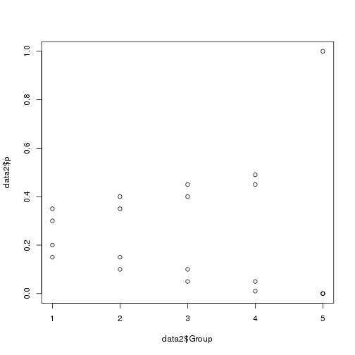
1 | #We can see that with increasing group number the allele frequencies become more divergent. |
Box C
Problem a
Given:
$$2d^2 = F_{ST} = \frac{\sigma^2}{\overline{p}\overline{q}}$$
$$p_1=0.5 + x; q_1=0.5 - x$$
$$p_2=0.5 - x; q_2=0.5 + x$$
Think of x as the distance from p=q=0.5 i.e the distance from maximum heterozygosity
So
$$\overline{p} = \frac{0.5 + x + 0.5 -x}{2}=\frac{1}{2}$$
$$\overline{q} = \frac{0.5 + x + 0.5 -x}{2}=\frac{1}{2}$$
$$F_{ST} = \frac{\sigma^2}{\frac{1}{2}\frac{1}{2}} = 4\sigma^2$$
We also know that $$d^2 = 1- \sqrt{p_1p_2} - \sqrt{q_1q_2}$$
$$= 1- \sqrt{(0.5+x)(0.5-x)} - \sqrt{(0.5-x)(0.5+x)}$$
$$= 1 - \sqrt{0.25 +0.5x -0.5x -x^2} - \sqrt{0.25 -0.5x +0.5x- x^2 }$$
$$= 1 - \sqrt{0.25-x^2} - \sqrt{0.25 -x^2 }$$
Substituting with the approximation $$\sqrt{0.25-x^2}=0.5-x^2$$
we get $$d^2 = 1- (0.5-x^2) - (0.5-x^2) = 2x^2$$
Multiply both sides by 2 to get $$2d^2=4x^2$$
$$2d^2 = 4x^2$$
1 | x <- c( 0.1, 0.2, 0.3, 0.35, 0.4, 0.49) |
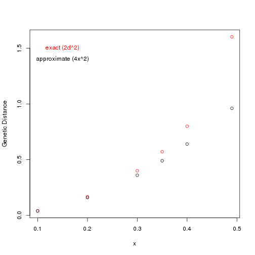
With small differences (x) in allele frequency, the approximate method is accurate.
For the trigonometry proof:
Realizing the sine is $$\frac{opposite}{hypotnuse}$$ and cosine is $$\frac{adjacent}{hypotnuse}$$
$$sin(\theta_1)=\frac{\sqrt{p_1}}{1}$$ and likewise $$sin(\theta_2) = \frac{\sqrt{p_2}}{1}$$
$$cos(\theta_1)=\frac{\sqrt{q_1}}{1}$$ and likewise $$cos(\theta_2) =\frac{ \sqrt{p_2}}{1}$$
$$cos(\theta_1 - \theta_2) = cos(\theta) = cos(\theta_1)cos(\theta_2) + sin(\theta_1)sin(\theta_2)$$
Substituting we get:
$$cos(\theta) = \sqrt{q_1q_2} + \sqrt{p_1p_2}$$
By definition:
$$d^2 = 1 - \sqrt{p_1p_2} - \sqrt{q_1q_2} = 1 - cos(\theta)$$
$$ChordLength = 2 \sqrt{\frac{1-cos(\theta)}{2}} = 2\sqrt{\frac{2}{4}}\sqrt{1-cos(\theta)} = \sqrt{2}\sqrt{1-cos(\theta)} = \sqrt{2}\sqrt{d^2} = d\sqrt{2}$$
Problem b
The R function dist() will calculate distance matrices using a variety of methods, none of which are the genetic distance we are interested in, exemplified by the equation:
$$d^2 = 1 - \sqrt{p_1p_2} - \sqrt{q_1q_2}$$
Therefore we need to define our own function “GeneticDistance”. I also represent the alleles as p.1 and p.2 only, to simplify the function.
1 | p.1 <- c(0.15, 0.25, 0.3, 0.4) |
## Box D ##
Problem a
$$\hat{F}=[ \frac{1}{2N}+(1-\frac{1}{2N})\hat{F} ](1-u)^2$$ $$\hat{F}=[\frac{1}{2N}+(\hat{F} -\frac{\hat{F}}{2N})](1-u)^2$$ $$\hat{F}=\frac{(1-u)^2}{2N}+ \hat{F}(1-u)^2 - \frac{\hat{F}}{2N}(1-u)^2$$ $$\hat{F} - \hat{F}(1-u)^2 + \frac{\hat{F}}{2N}(1-u)^2 =\frac{(1-u)^2}{2N}$$ $$\hat{F}[1-(1-u)^2 + \frac{(1-u)^2}{2N}]= \frac{(1-u)^2}{2N}$$ $$\hat{F} = \frac{(1-u)^2}{2N[1-(1-u)^2 + \frac{(1-u)^2}{2N}]}=\frac{(1-u)^2 }{2N-2N(1-u)^2+(1-u)^2}$$ $$\hat{F}=\frac{(1-u)^2}{2N} - \frac{(1-u)^2}{2N(1-u)^2} + \frac{(1-u)^2}{(1-u)^2}$$ $$\hat{F}=\frac{(1-u)^2}{2N} -\frac{1}{2N} + 1$$ $$\hat{F}=\frac{1}{2N}[(1-u)^2 - 1] + 1$$ $$\hat{F}=\frac{1}{2N[\frac{1}{(1-u)^2} - 1] + 1}$$ For the second part: $$\frac{1}{(1-u)^2} \approx 1+2u$$ Substitute into $$\hat{F}=\frac{1}{2N[\frac{1}{(1-u)^2} - 1] + 1}$$ to get $$\frac{1}{2N[1+2u-1]+1} = \frac{1}{2N[2u]+1} = \frac{1}{4Nu+1}$$Problem b
As in a only substitute m for u
Problem c
$$\hat{F}=[\frac{1}{2N}+(1-\frac{1}{2N})\hat{F}][1-(m+u)]^2$$
Substitute $$x = \frac{1}{2N}$$ and $$y=[1-(m+u)]^2$$ to get
$$\hat{F}=[x+(1-x)\hat{F}]y = [xy +(1-x)\hat{F}y]$$
$$\hat{F}=xy + \hat{F}y - \hat{F}yx = y(x + \hat{F} - \hat{F}x)$$
Rearrange to get $$\hat{F} - \hat{F}y + \hat{F}xy = xy$$
$$\displaystyle\hat{F}(1-y+xy) = xy$$
$$\displaystyle\hat{F} = \frac{xy}{1-y+xy} = \frac{1}{(\frac{1}{xy} - \frac{1}{x} +1)} = \frac{1}{\frac{1}{x}(\frac{1}{y}-1)+1}$$
Substitute in $$x = \frac{1}{2N}$$ and $$y=[1-(m+u)]^2$$ to get
$$\displaystyle\hat{F} = \frac{1}{2N[\frac{1}{1-(m+u)^2}-1]+1}$$
Using $$\displaystyle\frac{1}{1-(m+u)^2}\approx 1+2(m+u)$$ assuming m is not too large gives:
$$\displaystyle\hat{F} = \frac{1}{2N[1+2(m+u)-1]+1} = \frac{1}{2N[2(m+u)]+1} = \frac{1}{4N(m+u)+1}$$
Box E
Problem a
For a selectively neutral allele its fixation probability is $$\frac{1}{2N_a}$$ and its loss probability is $$1-\frac{1}{2N_a}$$
Fixation requires $4N_e$ generations, while loss requires $2(\frac{N_e}{N_a}ln(2N_A))$
For $$N_a=5000$$ and $$N_e$$ = 5000:
1 | N.a <- 5000 |
Problem b
For a selection coefficient s of 0.01:
1 | s <- 0.01 |
Problem c
The formula for the persistence of a harmful allele in a population is:
$$\displaystyle2\frac{N_e}{N_a}ln(\frac{2N_a}{2N_es})+1-\gamma$$
Where $$\gamma$$ is Euler’s constant. To obtain Euler’s constant we will use the negative derivative of the gamma function evaluated at 1: -digamma(1), which equals ~0.5772157
1 | s <- 0.01 |
i.e 8.148 generations.
Box F
Problem a
For the stepping stone model use $$\displaystyle\hat{F} \approx \frac{1}{4N\sqrt{2m\mu}+1}$$
For the island model use $$\displaystyle\hat{F} \approx \frac{1}{4N(m+\mu)+1}$$
1 | u <- 1e-6 |
Problem b
Using $$\displaystyle\hat{F} \approx \frac{1}{1 + 4\delta\sigma\sqrt{2\mu}}$$
and $$\delta = N$$ and $$\sigma=\sqrt{\mu}$$
1 | u <- 1e-6 |
Problem c
Using $$\displaystyle\hat{F} \approx \frac{1}{1 - 8\pi\delta\sigma^2/\ln(2\mu)}$$
1 | u <- 1e-6 |
Problem d
Comparing neighborhood sizes in b (uniform population distribution in one dimension) and c (uniform population distribution in two dimensions) above:
1 | u <- 1e-6 |
Box G
Problem a
$$\displaystyle p' = \frac{p(pw_{11} + qw_{12})}{\bar{w}}$$ Subtract p from both sides: $$\displaystyle p'-p = \frac{p(pw_{11} + qw_{12})}{\bar{w}}-p$$ Multiply p by$$\frac{\bar{w}}{\bar{w}}$$ and rearrange to get: $$\displaystyle \Delta p = \frac{1}{\bar{w}}[p(pw_{11} + qw_{12}) - p\bar{w} ]$$ Given that: $$\bar{w} = p^2w_{11} + 2pqw_{12} + q^2w_{22}$$ $$\displaystyle \Delta p = \frac{1}{\bar{w}}[p(pw_{11} + qw_{12}) - p(p^2w_{11} + 2pqw_{12} + q^2w_{22}) ]$$ $$\displaystyle \Delta p = \frac{1}{\bar{w}}[p^2w_{11} + pqw_{12} - pp^2w_{11} - 2p^2qw_{12} - pq^2w_{22} ]$$ $$\displaystyle \Delta p = \frac{1}{\bar{w}}[p^2w_{11} - pp^2w_{11} + pqw_{12} - 2ppqw_{12} - pq^2w_{22} ]$$ $$\displaystyle \Delta p = \frac{1}{\bar{w}}[w_{11}(p^2 - pp^2) + w_{12}(pq -2ppq) - pq^2w_{22} ]$$ $$\displaystyle \Delta p = \frac{1}{\bar{w}}[w_{11}p^2(1 - p) + w_{12}pq(1 -2p) - pq^2w_{22} ]$$ Given that $$1-2p=(1-p)-p=q-p$$: $$\displaystyle \Delta p = \frac{1}{\bar{w}}[w_{11}p^2q + w_{12}pq(q -p) - pq^2w_{22} ]$$ then factor out pq to get: $$\displaystyle \Delta p = \frac{pq}{\bar{w}}[w_{11}p + w_{12}(q -p) - qw_{22} ]$$ $$\displaystyle \Delta p = \frac{pq}{\bar{w}}[w_{11}p + w_{12}q -w_{12}p - qw_{22} ]$$ $$\displaystyle \Delta p = \frac{pq}{\bar{w}}[ p(w_{11} - w_{12}) +q(w_{12} - w_{22}) ]$$Problem b
Part 1
$$\displaystyle w_{11}=w_{12}=1 \;\;\; w_{22}=1-s$$ $$\displaystyle\frac{dp}{dt} = pq^2s$$ or rearrange to $$\displaystyle\frac{dp}{pq^2}=s\; dt$$ So from $$t_0$$ to $$t_1$$: $$\displaystyle\int_{p_0}^{p_t} \frac{1}{pq^2}dp = \int_{t_0}^{t_1} s\; dt$$ First the left hand integral. Given that: $$\displaystyle\int \frac{1}{x(1-x)^2}\;dx = \frac{1}{1-x}-ln(\frac{1-x}{x})$$ Then $$\displaystyle\int_{p_0}^{p_t} \frac{1}{pq^2}dp =[\frac{1}{1-p_t}-ln(\frac{1-p_t}{p_t})]-[\frac{1}{1-p_0}-ln(\frac{1-p_0}{p_0})]$$ $$\displaystyle =\frac{1}{1-p_t} - ln(\frac{1-p_t}{p_t})- \frac{1}{1-p_0} + ln(\frac{1-p_0}{p_0}) = \frac{1}{q_t} - ln(\frac{q_t}{p_t}) - \frac{1}{q_0} + ln(\frac{q_0}{p_0})$$ Because $$ln(\frac{a}{b}) = ln(a) - ln (b)$$ and $$ln(ab) = ln(a)+ln(b)$$ simplify to: $$\displaystyle = ln(\frac{p_tq_0}{p_0q_t}) + \frac{1}{q_t} - \frac{1}{q_0}$$ For the right hand integral: $$\displaystyle \int_{t_0}^{t_1} s\; dt = s(t - 0) = st$$ Setting the two solutions equal gives: $$\displaystyle st = ln(\frac{p_tq_0}{p_0q_t}) + \frac{1}{q_t} - \frac{1}{q_0}$$Part 2
$$\displaystyle \frac{dp}{dt} = \frac{pqs}{2}$$ rearrange to get:
$$\displaystyle 2\frac{1}{pq};dp = s;dt$$
Right hand side as above. For the left side:
$$\displaystyle 2\int^{p_t}_{p_0}\frac{1}{p(1-p)} dp$$ Given that $$\displaystyle \int \frac{1}{x(1-x)}\;dx = -ln\frac{(1-x)}{x}$$ $$\displaystyle 2\int^{p_t}_{p_0}\frac{1}{p(1-p)}\;dp = 2[[-ln\frac{1-p_t}{p_t}]-[-ln\frac{1-p_0}{p_0}]]$$ $$\displaystyle = 2[ ln\frac{p_t}{1-p_t} + ln\frac{1-p_0}{p_0}]$$ $$\displaystyle = 2[ ln\frac{p_t}{q_t} + ln\frac{q_0}{p_0}]$$ $$\displaystyle = 2 ln\frac{p_tq_0}{q_tp_0}$$ Part 3 $$\displaystyle \frac{dp}{dt} = p^2qs$$ rearrange to get: $$\displaystyle \frac{1}{p^2q}\;dp = s\;dt$$ Right hand side as above. We are also given that $$\displaystyle \int \frac{1}{x^2(1-x)}\;dx=-\frac{1}{x}-ln\frac{1-x}{x}$$ so: $$\displaystyle \int^{p_t}_{p_0}\frac{1}{p^2(1-p)}\;dp = -\frac{1}{p_t} - ln\frac{1-p_t}{p_t}-[-\frac{1}{p_0} - ln\frac{1-p_0}{p_0}]$$ $$\displaystyle = -\frac{1}{p_t} - ln\frac{q_t}{p_t} + \frac{1}{p_0} + ln\frac{q_0}{p_0}$$ $$\displaystyle = -\frac{1}{p_t} + \frac{1}{p_0} + ln\frac{p_t}{q_t} + ln\frac{q_0}{p_0}$$ $$\displaystyle = -\frac{1}{p_t} + \frac{1}{p_0} + ln\frac{p_tq_0}{q_tp_0}$$Part 4
Problem c
1 | #Part 1 |
Box H
Problem a
Given: $$P_t= P_{t-1}(1-\mu)+(1-P_{t-1})\nu$$We want the expression for: $P_t - \frac{\nu}{\mu+\nu}$ so subtract $\frac{\nu}{\mu+\nu}$ from both sides of the given equation.
$$p_t - \frac{\nu}{\mu+\nu} = p_{t-1}(1-\mu)+(1-p_{t-1})\nu - \frac{\nu}{\mu+\nu}$$ $$p_t - \frac{\nu}{\mu+\nu} = p_{t-1}- \mu p_{t-1} + \nu - \nu p_{t-1} - \frac{\nu}{\mu + \nu}$$ $$p_t - \frac{\nu}{\mu+\nu} = p_{t-1}(1 - \mu - \nu ) + \nu - \frac{\nu}{\mu + \nu}$$ $$p_t - \frac{\nu}{\mu+\nu} = p_{t-1}(1 - \mu - \nu ) + \frac{\nu(\mu + \nu)}{\mu + \nu} - \frac{\nu}{\mu + \nu}$$ $$p_t - \frac{\nu}{\mu+\nu} = p_{t-1}(1 - \mu - \nu ) + \frac{\nu\mu + \nu^2 - \nu}{\mu + \nu}$$ $$p_t - \frac{\nu}{\mu+\nu} = p_{t-1}(1 - \mu - \nu ) - \frac{\nu(1 - \mu - \nu)}{\mu + \nu}$$ $$p_t - \frac{\nu}{\mu+\nu} = [p_{t-1} - \frac{\nu}{\mu + \nu}](1 - \mu - \nu)$$ So $a=\frac{\nu}{\nu+\mu}$ and $b=(1-\mu-\nu)$ Given: $p_t - a = (p_0-a)b^t$ substitute to get: $$p_t - \frac{\nu}{\mu+\nu} = [p_0 - \frac{\nu}{\mu + \nu}](1 - \mu - \nu)^t$$ ### Problem b ### $$p_t = p_{t-1}(1-m)+\bar{p}m$$ We are interested in $p_t - \bar{p}$ so subtract $\bar{p}$ from both sides. $$p_t - \bar{p} = p_{t-1}(1-m)+\bar{p}m - \bar{p}$$ $$p_t - \bar{p} = p_{t-1}(1-m)+\bar{p}(m - 1)$$ $$p_t - \bar{p} = p_{t-1}(1-m)-\bar{p}(1 - m)$$ $$p_t - \bar{p} = (p_{t-1} - \bar{p})(1-m)$$ So $a=\bar{p}$ and $b=(1-m)$ $$p_t - \bar{p} = (p_{0} - \bar{p})(1-m)^t$$ Divide both sides by $\bar{p}$: $$\frac{p_t}{\bar{p}} - 1 = (\frac{p_0}{\bar{p}} -1)(1-m)^t$$ $$\frac{p_t}{\bar{p}} = (\frac{p_0}{\bar{p}} -1)(1-m)^t + 1$$ If $\frac{p_0}{\bar{p}}=2$, m=0.01, and t=69: $$\frac{p_t}{\bar{p}} = (2 -1)(1-0.01)^{69} + 1= 1.499$$
Problem c
Box I
A fitness is $w_{11}$a fitness is $w_{22}$
$$w=\frac{w_{11}}{w_{22}}$$ Given: $p_t = \frac{p_{t-1}w_{11}}{\bar{w}}$ and $q_t = \frac{q_{t-1}w_{22}}{\bar{w}}$ $$\frac{p_t}{q_t} = \frac{\frac{p_{t-1}w_{11}}{\bar{w}}}{\frac{q_{t-1}w_{22}}{\bar{w}}} = \frac{p_{t-1}w_{11}}{\bar{w}}\frac{\bar{w}}{q_{t-1}w_{22}} = \frac{p_{t-1}}{q_{t-1}}\frac{w_{11}}{w_{22}} = \frac{p_{t-1}}{q_{t-1}}w$$ Given: $\displaystyle \frac{p_t}{q_t}=\frac{p_0}{q_0}w^t$ take the natural ln of bothh sides:
Given: $\displaystyle ln(\frac{p_t}{q_t})=ln(\frac{p_0}{q_0}) + t ln(w)$
For a line y=mx + b where m=slope and b = y intercept
For the plot of $\displaystyle ln(\frac{p_t}{q_t})$ vs t:
Slope = m = $\displaystyle \frac{y_1-y_0}{x_1-x_0} = ln(w)$
Y intercept = b = $\displaystyle y_0 -mx_0= ln(\frac{p_0}{q_0})$
Two timepoints are given, call them $t_1$ and $t_2$
Use them to calculate the slope and y intercept. Then use the above equations to calculate $p_0$
1 | t.1 <- 5 |
Use $$\displaystyle \frac{p_t}{q_t}=\frac{p_0}{q_0}w^t$$ to calculate $$p_0$$
1 | #at t=5 |
Box J
For L(mutation):
L(mutation) = $$\displaystyle \mu$$ = 2e-6
$$\displaystyle \hat{q}=\sqrt{\frac{\mu}{s}}$$
1 | u <- 2e-6 |
L(segregation):
L(segregation) = (st)/(s+t)
$\hat{q}$= s/(s+t)
1 | s <- 1.04e-4 |
Box K
Problem a
At equilibrium $$w_1 = w_2$$
$$\theta -2p_1(1-p_1) = \theta -2p_2(1-p_2)$$
$$p_1(1-p_1) = \theta2p_2(1-p_2)$$
1 | n <- c(3,30,300) |
Problem b
If all frequencies are equal then $$p_i=p_j$$ and $$p=\frac{1}{n}$$
1 | n <- c(3,30,300) |
Box L
Problem a
1 | altitude <- c(259, 914,1402, 1890,2438, 2621, 3018) |
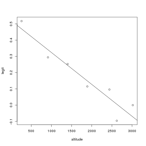
1 | #using y=mx + b where m:slope, b:y-intercept |
Problem b
1 | legit <- c(0.542, 0.401) |
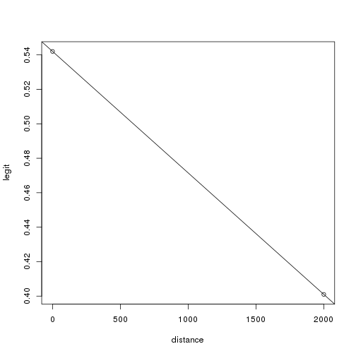
1 | #using y=mx + b where m:slope, b:y-intercept |