As I work with various packages related to text manipulation, I am beginning to realize what a mess the R package ecosystem can turn into. A variety of packages written by different contributers with no coordination amongst packages, overlapping functionality, colliding nomenclature. Many functions for “convenience” when base R could do the job. I also noticed this with packages like dplyr. I have commenced learning dplyr on multiple occasions only to find I don’t need it - I can do everything with base R without loading an extra package and learning new terminology. The problem I now encounter is that as these packages gain in popularity, code snippets and examples use them and I need to learn and understand the packages to make sense of the examples.
In my previous post on text manipulation I discussed the process of creating a corpus object. In this post I will investigate what can be done with a document term matrix. Starting with the previous post’s corpus:
1 |
|
There are a variety of methods available to inspect the dtmatrix:
1 | > dtm |
Note the sparsity is 81%. Remove sparse terms and inspect:
1 | > dtms <- removeSparseTerms(dtm, 0.1) # This makes a matrix that is 10% empty space, maximum. |
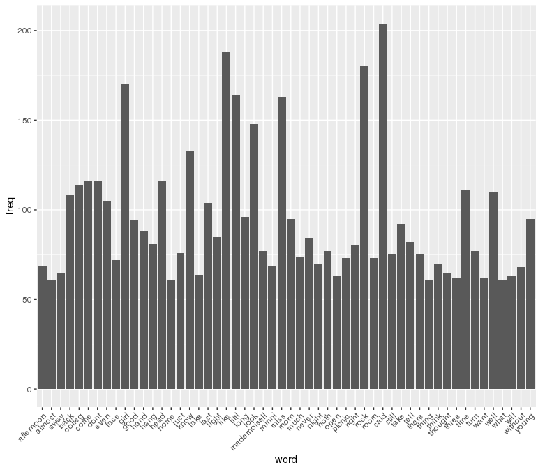
Now sparsity is down to 4%. Calculate word frequencies and plot as a histogram.
1 | > freq <- sort(colSums(as.matrix(dtm)), decreasing=TRUE) |
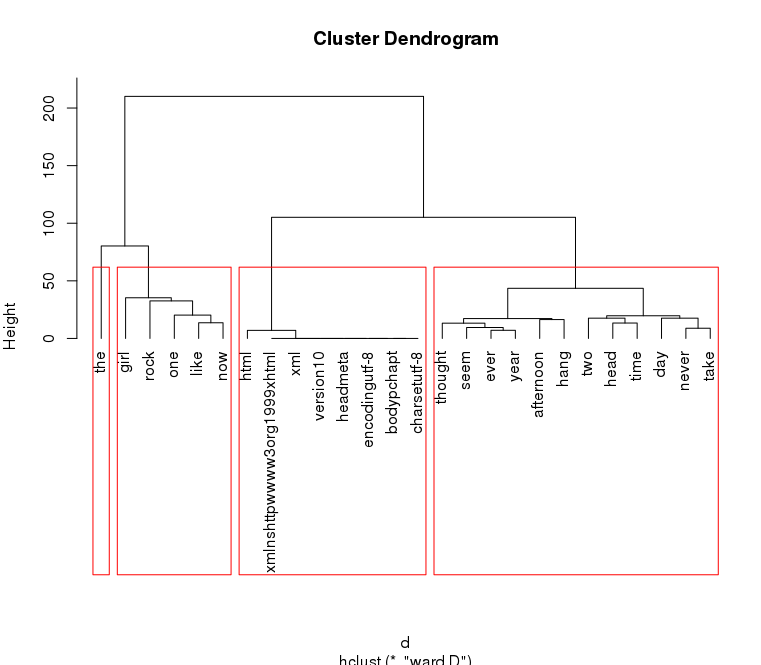
We can use hierarchal clustering to group related words. I wouldn’t read much meaning into this for Picnic, but it is comforting to see the xml/html terms clustering together in the third group - a sort of positive control.
1 |
|
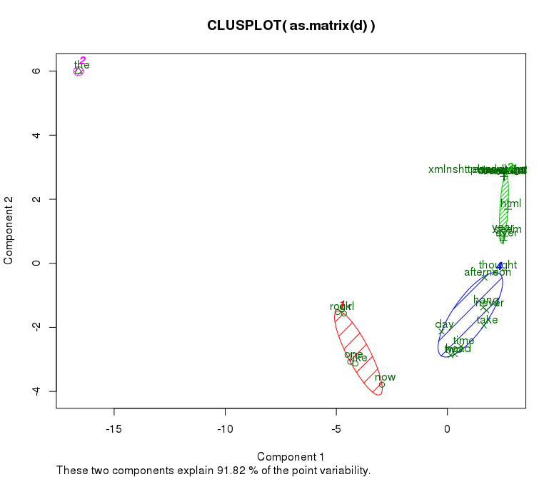
We can also use K-means clustering:
1 | library(fpc) |
Back here I didn’t mention that when creating the epub, it would display fine on my computer, but would not display on my Nook. A solution was to pass the file through Calibre. I diff’ed files coming out of Calibre with my originals but was not able to determine the minimum set of changes required for Nook compatibility. You can download the Calibre modified epub here, and the original here. If you determine what those Nook requirements are, please inform me.